Let’s pick up from where we left off in Part 1
Table of contents
- The
beforeRenderfunction - Value, Brightness, and Gamma Correction
- Waves
- Sawtooth Wave (Time)
- Triangle Wave
- Sine Wave
- Polar Waves
- Perlin Noise
- Next Steps
The beforeRender Function
While the render and render2D functions are called once for each pixel, the beforeRender function is called once before each new frame of pixels is rendered to the strip. This is where we can prepare any data needed by all of the pixels once.
The delta argument is the number of elapsed milliseconds (with a resolution of 6.25ns!) since the last time beforeRender was called. You can use delta to create animations that run at the same speed regardless of the frame rate.
In the introduction, we used the time function to make patterns move. In Part 1, we just did this in render, once for each pixel. Now we know that we should move that to beforeRender, since it only needs to be updated once per frame not once per pixel:
export function beforeRender(delta) {
  t = time(.1)
}

export function render2D(index, x, y) {
  h = x + t
  hsv(h, 1, 1)
}
Value, Brightness, and Gamma Correction
So far all of the patterns we’ve created turn on all the pixels at full brightness. Let’s add some variety.
Type (or copy and paste) the following code into the editor:
export function beforeRender(delta) {
  t = time(.1)
}

export function render2D(index, x, y) {
  v = x + t // scroll value horizontally
  v = v % 1 // wrap value from 1.0 to 0.0 (value does not wrap automatically)
  hsv(x, 1, v)
}
Note that we now have a static rainbow with a slightly dark line scrolling horizontally:
Value (v) is the amount of light energy. You might think that a value of 0.5 would be half as bright as 1.0, but humans actually perceive brightness on a power-law scale (search for “gamma correction” for more information). This means that our eyes perceive 0.25 as about half as bright as 1.0.
To make the value change more noticeable, let’s square it.
Change the line to the following:
hsv(x, 1, v * v)
Notice the value change is more pronounced? We’ve squared the value. Value is between 0.0 and 1.0. So a value of 0.5, for example, when squared becomes 0.25. A value of 0.6 becomes 0.36, etc. Squaring the fractional values increases the contrast.
Try cubing the value:
hsv(x, 1, v * v * v)
and the contrast increases even more. Notice that the brightest part stays just as bright, and the darkest part just as dark, but the values in between become more gradual. That’s because 1.0 cubed is still 1.0, and 0.0 cubed equals 0.0.
The final code:
export function beforeRender(delta) {
  t = time(.1)
}

export function render2D(index, x, y) {
  v = x + t // scroll value horizontally
  v = v % 1 // wrap value from 1.0 to 0.0 (value does not wrap automatically)
  v = v * v * v // increase contrast
  hsv(x, 1, v)
}
Waves
We’ve only been using the time function to add motion so far.
Let’s explore some different waveforms and how to generate them.
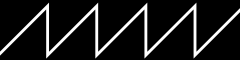
Sawtooth Wave (Time)
The time function that we’ve been using creates a sawtooth wave between 0.0 and 1.0 that loops about every 65.536 * interval seconds (use 0.015 for approximately 1 second).
Let’s use time to make a moving rainbow:
export function beforeRender(delta) {
  t = time(.1)
}

export function render2D(index, x, y) {
  h = x + t
  hsv(h, 1, 1)
}
We see it as a continuously scrolling rainbow, because the time wave wraps from 1.0 to 0.0, and red is at both ends of the rainbow (0.0 and 1.0).
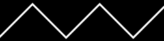
Triangle Wave
The triangle function converts a sawtooth wave between 0.0 and 1.0, like that returned by the time function, to a triangle wave between 0.0 and 1.0. The value passed to triangle is automatically wrapped between 0.0 and 1.0.
Add the following line inside the beforeRender function:
w = triangle(t)
And then change the first line in render2D:
h = x + w
The complete code:
export function beforeRender(delta) {
  t = time(.1)
  w = triangle(t)
}

export function render2D(index, x, y) {
  h = x + w
  hsv(h, 1, 1)
}
Notice now instead of constantly scrolling in one direction, it now moves back and forth!
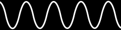
Sine Wave
The wave function converts a sawtooth wave between 0.0 and 1.0, like that returned by the time function, to a smooth sine wave between 0.0 and 1.0. The value passed to wave is automatically wrapped between 0.0 and 1.0.
Try changing line in beforeRender from triangle to wave:
w = wave(t)
The complete code:
export function beforeRender(delta) {
  t = time(.1)
  w = wave(t)
}

export function render2D(index, x, y) {
  h = x + w
  hsv(h, 1, 1)
}
Notice the wave moves back and forth more smoothly, slowing as it reaches the sides before reversing direction.
Polar Waves
Like in Part 1, we can switch from Cartesian XY coordinates to polar coordinates.
export function beforeRender(delta) {
  t = time(.1)
  w = wave(t)
}

export function render2D(index, x, y) {
  radius = hypot(x - .5, y - .5)
  h = radius + w
  v = 1
  hsv(h, 1, v)
}
Lets change it so the value moves but the hue doesn’t:
export function beforeRender(delta) {
  t = time(.1)
}

export function render2D(index, x, y) {
  radius = hypot(x - .5, y - .5)
  w = wave(t + radius)
  h = radius * 2
  v = w
  hsv(h, 1, v * v * v)
}
Flip the direction:
w = wave(t - radius)
The complete code:
export function beforeRender(delta) {
  t = time(.1)
}

export function render2D(index, x, y) {
  radius = hypot(x - .5, y - .5)
  w = wave(t - radius)
  h = radius * 2
  v = w
  hsv(h, 1, v * v * v)
}
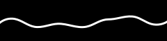
Perlin Noise
All of the above wave functions are symmetrical waveforms. Let’s explore a random, asymmetrical, irregular waveform.
perlin(x, y, z, seed)
The perlin function generates random 3D dimensional Perlin noise waveform. Every integer value produces a different random result, with smooth transitions between them. It returns a value ranging from -1.0 to 1.0.
Try this code:
export function beforeRender(delta) {
  t = time(7) // very slow sawtooth wave, cycles every 458.752 seconds!
  noiseTime = t * 256 // noise inputs range from 0 to 255
  n = perlin(noiseTime, 0, 0, 0) // perlin returns values ranging from -1.0 to 1.0
  n = (n * 0.5) + 0.5 // adjust them to 0.0 to 1.0
}

export function render2D(index, x, y) {
  h = x - n
  hsv(h, 1, 1)
}
Notice the rainbow now moves in a much less regular, predictable way.
Perlin is different in another way from the other waveforms we’ve tried so far: it’s a three-dimensional waveform! Lets use this to make a more interesting rainbow:
export function beforeRender(delta) {
  t = time(7)
  noiseTime = t * 256
}

export function render2D(index, x, y) {
  x2 = x + noiseTime
  y2 = y

  n = perlin(x2, y2, 0, 0) // perlin returns values ranging from -1.0 to 1.0
  n = (n * 0.5) + 0.5 // adjust them to 0.0 to 1.0
  h = n
  hsv(h, 1, 1)
}
We’ve mapped the three-dimensional Perlin noise waveform to the hues for each pixel, using the pixels’ two dimensional XY coordinates!
We can swap XY for polar coordinates:
export function beforeRender(delta) {
  t = time(7)
  noiseTime = t * 256
}

export function render2D(index, x, y) {
  radius = hypot(x - .5, y - .5)

  radians = atan2(y - .5, x - .5)
  angle = radians / PI / 2

  x2 = angle + noiseTime
  y2 = radius * 2

  n = perlin(x2, y2, 0, 0) // perlin returns values ranging from -1.0 to 1.0
  n = (n * 0.5) + 0.5 // adjust them to 0.0 to 1.0
  h = n
  hsv(h, 1, 1)
}
Next Steps
We’ll be back with more pattern tutorials! We’ll cover custom color palettes, to make going beyond rainbows easier!